User Guide

Installation

To install use pip:

# with imgui and jupyterlab
pip install -U "fastplotlib[notebook,imgui]"

# minimal install, install glfw, pyqt6 or pyside6 separately
pip install -U fastplotlib

# with imgui
pip install -U "fastplotlib[imgui]"

# to use in jupyterlab, no imgui
pip install -U "fastplotlib[notebook]"

We strongly recommend installing simplejpeg for use in notebooks, you must first install libjpeg-turbo.

• If you use conda, you can get libjpeg-turbo through conda.

• If you are on linux you can get it through your distro’s package manager.

• For Windows and Mac compiled binaries are available on their release page: libjpeg-turbo/libjpeg-turbo

Once you have libjpeg-turbo:

pip install simplejpeg

What is fastplotlib?

fastplotlib is a cutting-edge plotting library built using the pygfx rendering engine. The lower-level details of the rendering process (i.e. defining a scene, camera, renderer, etc.) are abstracted away, allowing users to focus on their data. The fundamental goal of fastplotlib is to provide a high-level, expressive API that promotes large-scale explorative scientific visualization. We want to make it easy and intuitive to produce interactive visualizations that are as performant and vibrant as a modern video game 😄

fastplotlib basics

Before giving a detailed overview of the library, here is a minimal example:

import fastplotlib as fpl
import imageio.v3 as iio

# create a `Figure`
fig = fpl.Figure()

# read data
data = iio.imread("imageio:astronaut.png")

# add image graphic
image_graphic = fig[0, 0].add_image(data=data)

# show the plot
fig.show()

if __name__ == "__main__":
    fpl.run()

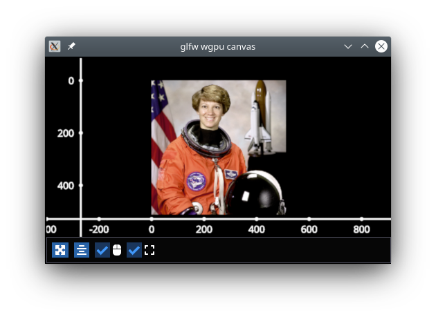
This is just a simple example of how the fastplotlib API works to create a plot, add some image data to the plot, and then visualize it. However, we are just scratching the surface of what is possible with fastplotlib. Next, let’s take a look at the building blocks of fastplotlib and how they can be used to create more complex visualizations.

Aside from this user guide, the Examples Gallery is the best place to learn specific things in fastplotlib. If you still need help don’t hesitate to post an issue or discussion post!

Figure

The starting point for creating any visualization in fastplotlib is a Figure object. This can be a single subplot or many subplots. The Figure object houses and takes care of the underlying rendering components such as the camera, controller, renderer, and canvas. Most users won’t need to use these directly; however, the ability to directly interact with the rendering engine is still available if needed.

By default, if no shape argument is provided when creating a Figure, there will be a single Subplot.

If a shape argument is provided, all subplots in a Figure can be accessed by indexing (i.e. fig_object[i ,j]). A “window layout” with customizable subplot positions and sizes can also be set by providing a rects or extents argument. The Examples Gallery has a few examples that show how to create a “Window Layout”.

After defining a Figure, we can begin to add Graphic objects.

Graphics

A Graphic can be an image, a line, a scatter, a collection of lines, and more. All graphics can also be given a convenient name. This allows graphics to be easily accessed from figures:

# create a `Figure`
fig = fpl.Figure()

# read data
data = iio.imread("imageio:astronaut.png")

add image graphic
image_graphic = fig[0, 0].add_image(data=data, name="astronaut")

# show figure
fig.show()

# index subplot to get graphic
fig[0, 0]["astronaut"]

# another way to index graphics in a subplot
fig[0, 0].graphics[0] is fig[0, 0]["astronaut"]  # will return `True`

See the examples gallery for examples on how to create and interactive with all the various types of graphics.

Graphics also have mutable properties. Some of these properties, such as the data or colors of a line can even be sliced, allowing for the creation of very powerful visualizations. Event handlers can be added to a graphic to capture changes to any of these properties.

1. Common properties that all graphics have

Feature Name	Description
name	Graphic name
offset	Offset position of the graphic, [x, y, z]
rotation	Graphic rotation quaternion
visible	Access or change the visibility
deleted	Used when a graphic is deleted, triggers events that can be useful to indicate this graphic has been deleted

2. Graphic-Specific properties

   1. ImageGraphic

   Feature Name	Description
   data	Underlying image data
   vmin	Lower contrast limit of an image
   vmax	Upper contrast limit of an image
   cmap	Colormap for a grayscale image, ignored if RGB(A)

   2. LineGraphic, LineCollection, LineStack

   Feature Name	Description
   data	underlying data of the line(s)
   colors	colors of the line(s)
   cmap	colormap of the line(s)
   thickness	thickness of the line(s)

   3. ScatterGraphic

   Feature Name	Description
   data	underlying data of the scatter points
   colors	colors of the scatter points
   cmap	colormap of the scatter points
   sizes	size of the scatter points

   4. TextGraphic

   Feature Name	Description
   text	data of the text
   font_size	size of the text
   face_color	color of the text face
   outline_color	color of the text outline
   outline_thickness	thickness of the text

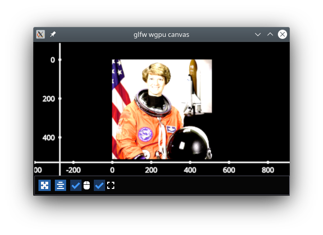
Using our example from above: once we add a Graphic to the figure, we can then begin to change its properties.

image_graphic.vmax = 150

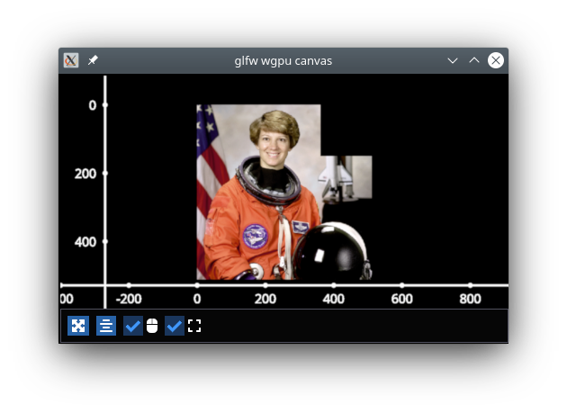
Graphic properties also support numpy-like slicing for getting and setting data. For example

# basic numpy-like slicing, set the top right corner
image_graphic.data[:150, -150:] = 0

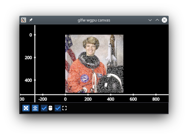
Fancy indexing is also supported!

bool_array = np.random.choice([True, False], size=(512, 512), p=[0.1, 0.9])
image_graphic.data[bool_array] = 254

Selectors

A primary feature of fastplotlib is the ability to easily interact with your data. Two extremely helpful tools that can be used in order to facilitate this process are a LinearSelector and LinearRegionSelector.

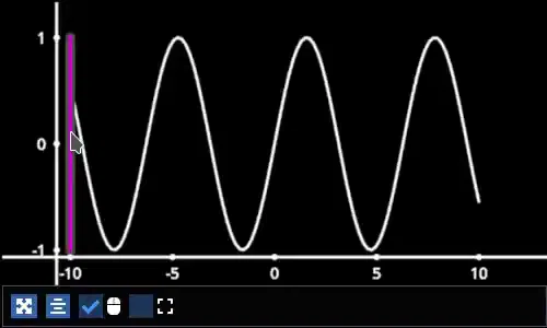
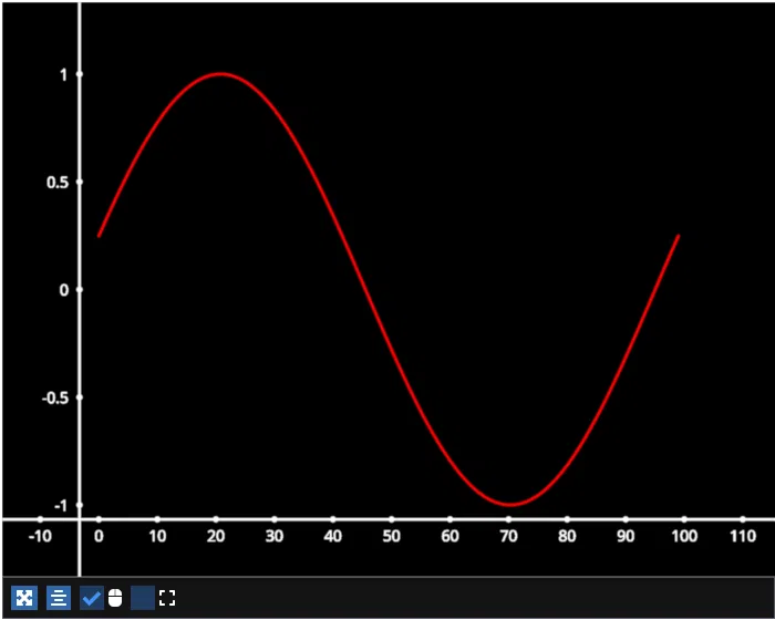
A LinearSelector is a horizontal or vertical line slider. This tool allows you to very easily select different points in your data. Let’s look at an example:

import fastplotlib as fpl
import numpy as np

# generate data
xs = np.linspace(-10, 10, 100)
ys = np.sin(xs)
sine = np.column_stack([xs, ys])

fig = fpl.Figure()

sine_graphic = fig[0, 0].add_line(data=sine, colors="w")

# add a linear selector the sine wave
selector = sine_graphic.add_linear_selector()

fig.show(maintain_aspect=False)

A LinearRegionSelector is very similar to a LinearSelector but as opposed to selecting a singular point of your data, you are able to select an entire region.

See the examples gallery for more in-depth examples with selector tools.

Now we have the basics of creating a Figure, adding Graphics to a Figure, and working with Graphic properties to dynamically change or alter them.

Events

Events can be a multitude of things: canvas events such as mouse or keyboard events, or events related to Graphic properties.

There are two ways to add events to a graphic:

1. Use the method add_event_handler()

   def event_handler(ev):
       pass
   
   graphic.add_event_handler(event_handler, "event_type")
   

2. or a decorator

   @graphic.add_event_handler("event_type")
   def event_handler(ev):
       pass
   

The event_handler is a user-defined callback function that accepts an event instance as the first and only positional argument. Information about the structure of event instances are described below. The "event_type" is a string that identifies the type of event.

graphic.supported_events will return a tuple of all event_type strings that this graphic supports.

When an event occurs, the user-defined event handler will receive an event object. Depending on the type of event, the event object will have relevant information that can be used in the callback. See the next section for details.

Graphic property events

All Graphic events are instances of fastplotlib.GraphicFeatureEvent and have the following attributes:

attribute	type	description
type	str	name of the event type
graphic	Graphic	graphic instance that the event is from
info	dict	event info dictionary
target	WorldObject	pygfx rendering engine object for the graphic
time_stamp	float	time when the event occurred, in ms

Selectors have one event called selection which has extra attributes in addition to those listed in the table above. The selection event section covers these.

The info attribute for most graphic property events will have one key, "value", which is the new value of the graphic property. Events for graphic properties that represent arrays, such the data properties for images, lines, and scatters will contain more entries. Here are a list of all graphic properties that have such additional entries:

• ImageGraphic

  • data

• LineGraphic

  • data, colors, cmap

• ScatterGraphic

  • data, colors, cmap, sizes

You can understand an event’s attributes by adding a simple event handler:

@graphic.add_event_handler("event_type")
def handler(ev):
    print(ev.type)
    print(ev.graphic)
    print(ev.info)

# trigger the event
graphic.event_type = <new data>

# direct example
@image_graphic.add_event_handler("cmap")
def cmap_changed(ev):
    print(ev.type)
    print(ev.info)

image_graphic.cmap = "viridis"
# this will trigger the cmap event and print the following:
# 'cmap'
# {"value": "viridis"}

The Event Tables provide a description of the event info dicts for all Graphic Feature Events.

Selection event

The selection event for selectors has additional attributes, mostly callable methods, that aid in using the selector tool, such as getting the indices or data under the selection. The info dict will contain one entry value which is the new selection value.

The Event Tables provide a description of the additional attributes as well as the event info dicts for selector events.

Canvas Events

Canvas events can be added to a graphic or to a Figure (see next section). Here is a description of all canvas events and their attributes.

The examples gallery provides several examples using pointer and key events.

Pointer events

List of pointer events:

• pointer_down: emitted when the user interacts with mouse,

• pointer_up: emitted when the user releases a pointer.

• pointer_move: emitted when the user moves a pointer. This event is throttled.

• click: emmitted when a mouse button is clicked.

• double_click: emitted on a double-click. This event looks like a pointer event, but without the touches.

• wheel: emitted when the mouse-wheel is used (scrolling), or when scrolling/pinching on the touchpad/touchscreen.

  Similar to the JS wheel event, the values of the deltas depend on the platform and whether the mouse-wheel, trackpad or a touch-gesture is used. Also, scrolling can be linear or have inertia. As a rule of thumb, one “wheel action” results in a cumulative dy of around 100. Positive values of dy are associated with scrolling down and zooming out. Positive values of dx are associated with scrolling to the right. (A note for Qt users: the sign of the deltas is (usually) reversed compared to the QWheelEvent.)

  On MacOS, using the mouse-wheel while holding shift results in horizontal scrolling. In applications where the scroll dimension does not matter, it is therefore recommended to use delta = event[‘dy’] or event[‘dx’].

  • dx: the horizontal scroll delta (positive means scroll right).

  • dy: the vertical scroll delta (positive means scroll down or zoom out).

  • x: the mouse horizontal position during the scroll.

  • y: the mouse vertical position during the scroll.

  • buttons: a tuple of buttons being pressed down.

  • modifiers: a tuple of modifier keys being pressed down.

  • time_stamp: a timestamp in seconds.

All pointer events have the following attributes:

• x: horizontal position of the pointer within the widget.

• y: vertical position of the pointer within the widget.

• button: the button to which this event applies. See “Mouse buttons” section below for details.

• buttons: a tuple of buttons being pressed down (see below)

• modifiers: a tuple of modifier keys being pressed down. See section below for details.

• ntouches: the number of simultaneous pointers being down.

• touches: a dict with int keys (pointer id’s), and values that are dicts that contain “x”, “y”, and “pressure”.

• time_stamp: a timestamp in seconds.

Mouse buttons:

• 0: No button.

• 1: Left button.

• 2: Right button.

• 3: Middle button

• 4-9: etc.

Key events

List of key (keyboard keys) events:

• key_down: emitted when a key is pressed down.

• key_up: emitted when a key is released.

Key events have the following attributes:

• key: the key being pressed as a string. See section below for details.

• modifiers: a tuple of modifier keys being pressed down.

• time_stamp: a timestamp in seconds.

The key names follow the browser spec.

• Keys that represent a character are simply denoted as such. For these the case matters: “a”, “A”, “z”, “Z” “3”, “7”, “&”, “ “ (space), etc.

• The modifier keys are: “Shift”, “Control”, “Alt”, “Meta”.

• Some example keys that do not represent a character: “ArrowDown”, “ArrowUp”, “ArrowLeft”, “ArrowRight”, “F1”, “Backspace”, etc.

Time stamps

Since the time origin of time_stamp values is undefined, time stamp values only make sense in relation to other time stamps.

Add canvas event handlers to a Figure

You can add event handlers to a Figure object’s renderer. For example, this is useful for defining click events where you want to map click positions to the nearest graphic object. See the previous section for a description of all the canvas events.

Renderer event handlers can be added using a method or a decorator.

For example:

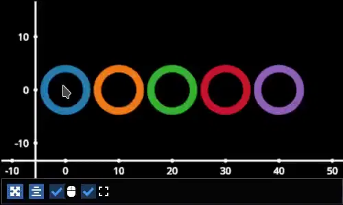
import fastplotlib as fpl
import numpy as np

# generate some circles
def make_circle(center, radius: float, n_points: int = 75) -> np.ndarray:
    theta = np.linspace(0, 2 * np.pi, n_points)
    xs = radius * np.sin(theta)
    ys = radius * np.cos(theta)

    return np.column_stack([xs, ys]) + center

# this makes 5 circles, so we can create 5 cmap values, so it will use these values to set the
# color of the line based by using the cmap as a LUT with the corresponding cmap_value
circles = list()
for x in range(0, 50, 10):
    circles.append(make_circle(center=(x, 0), radius=4, n_points=100))

# create figure
fig = fpl.Figure()

# add circles to plot
circles_graphic = fig[0,0].add_line_collection(data=circles, cmap="tab10", thickness=10)

# get the nearest graphic that is clicked and change the color
@fig.renderer.add_event_handler("click")
def click_event(ev):
    # reset colors
    circles_graphic.cmap = "tab10"

    # map the click position to world coordinates
    xy = fig[0, 0].map_screen_to_world(ev)[:-1]

    # get the nearest graphic to the position
    nearest = fpl.utils.get_nearest_graphics(xy, circles_graphic)[0]

    # change the closest graphic color to white
    nearest.colors = "w"

fig.show()

Integrating with UI libraries

After you are comfortable with creating graphics, changing their properties, and creating events, you can easily integrate fastplotlib with common UI libraries such as ipywidgets, Qt, and imgui. wx should also work but this is not thoroughly tested.

ipywidgets

The ipywidgets library is great for rapidly building UIs for prototyping in jupyter. It is particularly useful for scientific and engineering applications since we can rapidly create a UI to interact with our fastplotlib visualization. The main downside is that it only works in jupyter.

For examples please see the examples gallery.

Qt

Qt is a very popular UI library written in C++, PyQt6 and PySide6 provide python bindings. There are countless tutorials on how to build a UI using Qt which you can easily find if you google PyQt. You can embed a Figure as a Qt widget within a Qt application.

For examples please see the examples gallery.

imgui

Imgui is also a very popular library used for building UIs. The difference between imgui and ipywidgets, Qt, and wx is the imgui UI can be rendered directly on the same canvas as a fastplotlib Figure. This is hugely advantageous, it means that you can write an imgui UI and it will run on any GUI backend, i.e. it will work in jupyter, Qt, glfw and wx windows! The programming model is different from Qt and ipywidgets, there are no callbacks, but it is easy to learn if you see a few examples.

We specifically use imgui-bundle for the python bindings in fastplotlib. There is large community and many resources out there on building UIs using imgui.

To install fastplotlib with imgui use the imgui extras option, i.e. pip install fastplotlib[imgui], or pip install imgui_bundle if you’ve already installed fastplotlib.

Fastplotlib comes built-in with imgui UIs for subplot toolbars and a standard right-click menu with a number of options. You can also make custom GUIs and embed them within the canvas, see the examples gallery for detailed examples.

Some tips:

The imgui-bundle docs as of March 2025 don’t have a nice API list (as far as I know), here is how we go about developing UIs with imgui:

1. Use the pyimgui API docs to locate the type of UI element we want, for example if we want a slider_int: https://pyimgui.readthedocs.io/en/latest/reference/imgui.core.html#imgui.core.slider_int

2. Look at the function signature in the imgui-bundle sources. You can usually access this easily with your IDE: pthom/imgui_bundle

3. pyimgui and imgui-bundle sometimes don’t have the same function signature, so we use a combination of the pyimgui docs and imgui-bundle function signature to understand and implement the UI element.

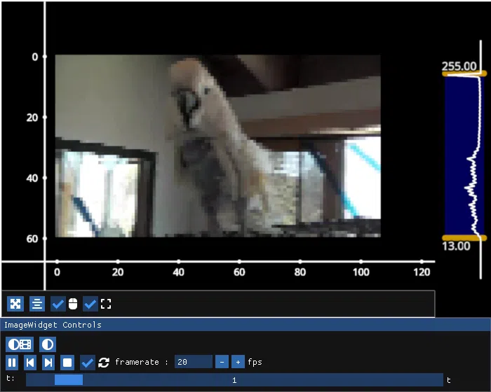
ImageWidget

Often times, developing UIs for interacting with multi-dimension image data can be tedious and repetitive. In order to aid with common image and video visualization requirements the ImageWidget automatically generates sliders to easily navigate through different dimensions of your data. The image widget supports 2D, 3D and 4D arrays.

Let’s look at an example:

import fastplotlib as fpl
import imageio.v3 as iio

movie = iio.imread("imageio:cockatoo.mp4")

iw_movie = ImageWidget(
    data=movie,
    rgb=True
)

iw_movie.show()

Animations

An animation function is a user-defined function that gets called on every rendering cycle. Let’s look at an example:

import fastplotlib as fpl
import numpy as np

# generate some data
start, stop = 0, 2 * np.pi
increment = (2 * np.pi) / 50

# make a simple sine wave
xs = np.linspace(start, stop, 100)
ys = np.sin(xs)

figure = fpl.Figure(size=(700, 560))

# plot the image data
sine = figure[0, 0].add_line(ys, name="sine", colors="r")


# increment along the x-axis on each render loop :D
def update_line(subplot):
    global increment, start, stop
    xs = np.linspace(start + increment, stop + increment, 100)
    ys = np.sin(xs)

    start += increment
    stop += increment

    # change only the y-axis values of the line
    subplot["sine"].data[:, 1] = ys


figure[0, 0].add_animations(update_line)

figure.show(maintain_aspect=False)

Here we are defining a function that updates the data of the LineGraphic in the plot with new data. When adding an animation function, the user-defined function will receive a subplot instance as an argument when it is called.

Spaces

There are several spaces to consider when using fastplotlib:

1. World Space

   World space is the 3D space in which graphical objects live. Objects and the camera can exist anywhere in this space.

2. Data Space

   Data space is simply the world space plus any offset or rotation that has been applied to an object.

Note

World space does not always correspond directly to data space, you may have to adjust for any offset or rotation of the Graphic.

3. Screen Space

   Screen space is the 2D space in which your screen pixels reside. This space is constrained by the screen width and height in pixels. In the rendering process, the camera is responsible for projecting the world space into screen space.

Note

When interacting with Graphic objects, there is a very helpful function for mapping screen space to world space (Figure.map_screen_to_world(pos=(x, y))). This can be particularly useful when working with click events where click positions are returned in screen space but Graphic objects that you may want to interact with exist in world space.

For more information on the various spaces used by rendering engines please see this article

Using fastplotlib in an interactive shell

There are multiple ways to use fastplotlib in interactive shells, such as ipython.

1. Jupyter

On jupyter lab the jupyter backend (i.e. jupyter_rfb) is normally selected. This works via client-server rendering. Images generated on the server are streamed to the client (Jupyter) via a jpeg byte stream. Events (such as mouse or keyboard events) are then streamed in the opposite direction prompting new images to be generated by the server if necessary. This remote-frame-buffer approach makes the rendering process very fast. fastplotlib viusalizations can be displayed in cell output or on the side using sidecar.

A Qt backend can also optionally be used as well. If %gui qt is selected before importing fastplotlib then this backend will be used instead.

Lastly, users can also force using glfw by specifying this as an argument when instantiating a Figure (i.e. Figure(canvas="gflw").

Note

Do not mix between gui backends. For example, if you start the notebook using Qt, do not attempt to force using another backend such as jupyter_rfb later.

2. IPython

Users can select between using a Qt backend or gflw using the same methods as above.