
NDWidget and Systems Neuroscience Datasets#

Binned spikes of a neuropixel recording in conjunctions with spectrograms of vocalizations and Gerbil behavior. Data from Gily Ginosar, Dan Sanes lab, NYU.#

Quality assessment using behavior data processed by Lightning Pose, showing the behavior video with tracks, predicted lightning actions and likelihood scores. Data from Kcénia Bougrova, IBL & Champalimaud Foundation, Mainen Lab.#

A systems neuroscience session can produce many n-dimensional arrays. A multi-plane, multi-FOV calcium imaging movie has dimensions for the FOV, plane, time, rows and columns. Alongside it there may be electrophysiology recordings, videos from several behavior cameras, the keypoints tracked in each video, and behavioral labels. Each of these comes from its own acquisition system with its own shape, dimension order and sampling rate, such as 30 Hz for a behavior camera, 30 kHz for an electrophysiology probe, and a few Hz for each imaging plane.
The NDWidget provides a declarative interface for interacting with large volumes of this data, with ease and at
speed. For each array you name its dimensions and declare which of them are drawn. Arrays that share a dimension
name stay in sync, whatever their shape, dimension order or sampling rate. The widget works out the rest: a slider
for every dimension that is not drawn, the mapping from a slider position onto each array’s own indices, windowing,
asynchronous reads, and which graphics need to update.
We built the NDWidget for:
better quality control of experimental data
prototyping new analysis ideas and algorithms
analysis pipeline agnostic visualizations
visualizing large datasets on the remote infrastructure where the analysis usually happens
developing new scientific insights by exploring all of the modalities together
Any n-dimensional data, any graphical representation#
Each array is added with two declarations. dims names every dimension of the array, in the order in which it
appears in the array, and display_dims names the dimensions that are drawn, in display order. Every other
dimension becomes a slider:
# a multi-plane calcium imaging movie, [time, plane, rows, cols]
ndw["movie"].add_nd_image(
    movie,
    dims=("time", "plane", "m", "n"),
    display_dims=("m", "n"),  # "time" and "plane" become sliders
)
With display_dims=("plane", "m", "n") the same movie is drawn as a volume, and only "time" is a slider.
Positional data, such as traces or keypoints, is an array of shape [..., l, p, d], where l is the number of
lines, scatters or heatmap rows, p is the number of datapoints in each of them, often timepoints, and d holds
the (x, y) or (x, y, z) coordinate of each datapoint. p is both drawn and given a slider, and the widget draws a
window of p around the slider position.
method |
draws |
|---|---|
|
grayscale or RGB(A) images and volumes, such as calcium imaging movies |
|
video frames, with the YUV components sent straight to the GPU, such as behavior videos |
|
stacked lines, lines, scatters or a heatmap on a time axis, such as traces, spike rasters, spectrograms and ethograms |
|
scatters, such as tracked keypoints |
|
lines, such as keypoint trajectories |
|
vectors |
Several of these can share a subplot, such as keypoints drawn over the video they were tracked in.
add_nd_timeseries draws a LineStack by default. The graphical representation of positional data is not
fixed by its shape, and graphic_type can be changed while the widget is running, from code or from the
right-click menu of the graphic:
ndg = ndw["traces"].add_nd_timeseries(
    traces,  # [cell, time, xy]
    dims=("cell", "time", "xy"),
    display_dims=("cell", "time", "xy"),
)

ndg.graphic_type = fpl.ImageGraphic  # the same traces as a heatmap
The data does not have to be a numpy array. Anything with dtype, ndim, shape and __getitem__ can be
used, such as a zarr or HDF5 dataset, a torch tensor, or a lazy reader of your own. The data can even be a function
of the index: an object whose __getitem__ computes the requested slice is used in the same way, such as a calcium
imaging movie that is computed from a matrix factorization one frame at a time. For any other data source, subclass
the slicer for that representation, NDImageSlicer for images or NDPositionsSlicer for positional data, and
implement get, which is given the current slider positions and returns the slice to draw.
fastplotlib.nds_extras.pandas.PandasSlicer reads the coordinates from the columns of a pandas.DataFrame, so
pose tracking output can be used directly.
Different sampling rates, any dim order#
A slider position is not an array index. It is a value in reference units, the scientific units of that dimension,
such as seconds or depth in microns. Each slider dimension is given a range in these units, and step is the
increment used by the step buttons and by playback:
ndw = fpl.NDWidget(
    ranges={"time": (0.0, 600.0, 1 / 30)},  # (start, stop, step) in seconds
    shape=(1, 2),
    names=["video", "ephys"],
)
Each array maps a slider position onto its own indices with slider_maps. An array of reference values, such as
the timestamp of every frame or sample, is used through its searchsorted, and a callable can be given for any
other mapping:
ndw["video"].add_video(
    video,
    dims=("time", "m", "n"),
    display_dims=("m", "n"),
    slider_maps={"time": frame_times},  # seconds, one per video frame
)

ndw["ephys"].add_nd_timeseries(
    traces,  # [channel, time, xy]
    dims=("channel", "time", "xy"),
    display_dims=("channel", "time", "xy"),
    slider_maps={"time": sample_times},  # seconds, one per sample
)
A slider position of 30 seconds resolves to frame 3,000 of a 100 Hz video and to sample 600,000 of a 20 kHz recording. Nothing is resampled onto a common rate, and no modality is expressed in the indices of another.
Dimensions are matched by name, so the arrays can have any number of dimensions in any order. An array declared as
("col", "depth", "row", "time") and displayed as ("row", "col") is transposed for you, and it shares the
"time" and "depth" sliders with every other array that has those dimensions. Different names keep timelines
apart: two recording sessions whose time dimensions are named "time-s1" and "time-s2" get a slider each, in
the same widget.
The current slider positions are ndw.indices. Moving a slider, playback, the step buttons, and dragging the line
that marks the current time in a timeseries subplot all change it, and it can be set programmatically:
ndw.indices = {"time": 12.5} # moves the sliders and updates every NDGraphic with a time dimension
Several widgets can share one set of sliders, which spreads a session across separate windows:
ndw_behavior = fpl.NDWidget(
    ranges={"time": (0.0, 600.0, 1 / 30)},
    shape=(1, 2),
    names=["camera-left", "camera-right"],
)

ndw_ephys = fpl.NDWidget(indices=ndw_behavior.indices, names=["ephys"])
Window functions#
A window function reduces a slider dimension over a window around the current position, such as a rolling mean, a
rolling median, a maximum projection or a Gaussian smoothing. The window size is in reference units, and any function
that takes axis and keepdims can be used:
ndw["movie"].add_nd_image(
    movie,  # [time, plane, rows, cols]
    dims=("time", "plane", "m", "n"),
    display_dims=("m", "n"),
    slider_maps={"time": frame_times},
    window_funcs={"time": (np.mean, 2.5)},  # mean over 2.5 seconds around the current time
    window_order=("time",),
)
Only the dimensions in window_order are windowed, in that order. spatial_func is applied to the slice after
the window functions, such as a spatial Gaussian filter, and datapoints_window_func applies a window function
along the datapoints of positional data, such as smoothing a trace.
For positional data, display_window sets the window of datapoints that is drawn around the current position, in
reference units, such as 10 seconds of traces. Only that window is sent to the GPU, so the array can be much larger
than GPU memory. Panning or zooming a timeseries subplot moves and resizes the display window.
Asynchronous reads and CUDA arrays#
When a slider moves, the widget schedules a fetch on every NDGraphic that has that dimension. Fetches are
asynchronous tasks on the render loop. While a slider is dragged, fetches for positions that have already been
passed are skipped, so the drag stays responsive on data that cannot be read at frame rate. Playback, the step
buttons and ndw.indices queue their fetches instead, and each one is drawn in order.
A data object whose __getitem__ returns a future, such as an
asyncvideo reader that decodes frames in its own process, is awaited
without blocking the render loop. For numpy arrays, window functions and spatial_func run in a thread pool.
CUDA arrays, such as torch tensors, stay on the GPU while they are sliced and windowed. Window functions and
spatial_func are applied to them directly, so they should run on the GPU, for example written with torch, and only
the slice that is drawn is copied to host memory, in the thread pool, before it is uploaded for rendering. CUDA work
is itself asynchronous, so lazy GPU compute does not block the visualization. For example, an array that
reconstructs a calcium imaging movie from a matrix factorization on the GPU computes each frame as you scroll to it.
We are currently working on direct within-GPU transfer of data from CUDA to the renderer, with no host roundtrip.
Desktop, notebooks and remote#
The same code runs everywhere. A script or application can use Qt, glfw, or wx:
ndw.show()

if __name__ == "__main__":
    fpl.loop.run()
In a notebook, such as Jupyter, marimo or VS Code, ndw.show() as the last line of a cell puts the widget in the
output cell. Remote rendering can also be streamed over http. With uvicorn installed, the address is printed when
the server starts:
RENDERCANVAS_BACKEND=http python viewer.py
In a notebook and over http, the rendering is done on the machine that runs Python, and the browser receives a stream of rendered frames. The data never leaves that machine, so large datasets can be visualized on the remote infrastructure where the analysis happens. The sliders, playback controls and menus of the widget are drawn on the canvas, so they are the same in every environment. We are currently working on faster remote rendering.
Built on WGPU, with few dependencies#
fastplotlib is built on the pygfx rendering engine, which is powered by
WGPU, the cross-platform modern GPU API. WGPU runs on Windows, Linux and
Mac via DX12, Vulkan, or Metal, and is the de facto successor to older OpenGL. Everything the NDWidget draws is
rendered through WGPU, including its sliders and menus.
fastplotlib depends on numpy, pygfx, wgpu and cmap, and the NDWidget also requires
imgui-bundle. See the user guide for installation instructions.
Example: a multi-modal viewer#
This example builds a viewer for one session with calcium imaging, two behavior cameras read with asyncvideo, keypoints tracked with Lightning Pose, and an ethogram built with lightning actions. The imaging was demixed with masknmf, whose results include the denoised movie and the movies of the demixed signal, the residual and the background, each computed on the GPU one frame at a time. Every modality comes with the timestamp of each of its samples, in seconds on the session clock:
ndw = fpl.NDWidget(ranges={"time": (start_time, stop_time, step)})

ndw["pmd"].add_nd_image(
    pmd_array,  # [time, m, n]
    dims=("time", "m", "n"),
    display_dims=("m", "n"),
    slider_maps={"time": ca_timestamps},  # [2050.02, 2050.22, 2050.42, ...]
)

# demixed_movie, residual_movie and background_movie are added in the same way

The traces and the ethogram are timeseries, and the ethogram is drawn as a heatmap:
ndw["traces"].add_nd_timeseries(
    traces,  # [n_neurons, time, xy]
    dims=("l", "time", "d"),
    display_dims=("l", "time", "d"),
    slider_maps={"time": ca_timestamps},
)

ndw["ethogram"].add_nd_timeseries(
    ethogram,  # a probability distribution per timepoint, from lightning actions
    dims=("l", "time", "d"),
    display_dims=("l", "time", "d"),
    graphic_type=fpl.ImageGraphic,
    slider_maps={"time": left_cam_timestamps},
)

Each video is added with its own frame timestamps, and the keypoints are drawn over the left camera from the columns of the Lightning Pose DataFrame:
ndw["behavior-left"].add_video(
    video_left,  # [time, m, n], the YUV components are sent straight to the GPU
    dims=("time", "m", "n"),
    display_dims=("m", "n"),
    slider_maps={"time": left_cam_timestamps},  # [2049.994, 2050.011, 2050.027, ...]
)

# video_right is added in the same way, with right_cam_timestamps

ndw["behavior-left"].add_nd_scatter(
    keypoints_dataframe,
    dims=("l", "time", "d"),
    display_dims=("l", "time", "d"),
    slicer=fpl.nds_extras.pandas.PandasSlicer,
    slicer_kwargs={"columns": keypoint_columns},  # [("paw_l_x", "paw_l_y"), ("nose_tip_x", "nose_tip_y"), ...]
    display_window=0,  # only the keypoints of the current frame
    slider_maps={"time": left_cam_timestamps},
)
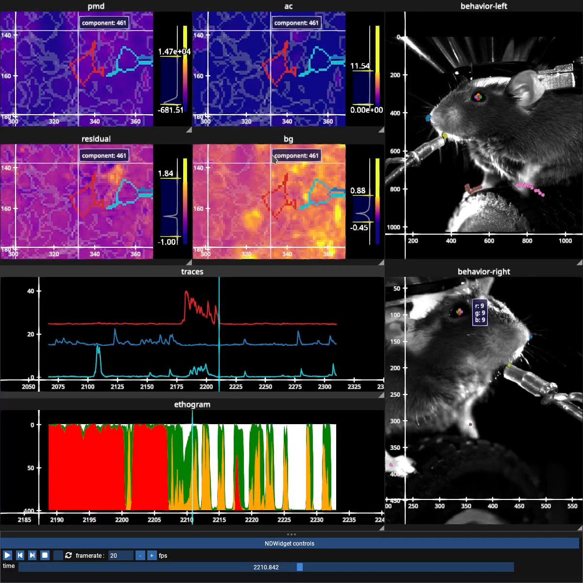
This is only a very simple example. The NDWidget is built to handle an arbitrary number of heterogeneously
sampled arrays, with dimensions in any order. For example, we could have multiple sessions that we can represent as
different timelines, and volumetric recordings with depth, etc.
ndw = fpl.NDWidget(
    ranges={
        "time-s1": (start_s1, start_s2, step),  # session 1
        "time-s2": (start_s2, start_s3, step),  # session 2
        "depth": (start_z, end_z, step_z),  # microns
    }
)

# specify the associated timeline when adding each NDGraphic
ndw["pmd-s1"].add_nd_image(
    pmd_array_s1,  # [time, z, m, n]
    dims=("time-s1", "depth", "m", "n"),
    display_dims=("m", "n"),
    slider_maps={"time-s1": ca_timestamps_s1, "depth": plane_depths},  # plane_depths: [0.0, 20.0, 40.0, ...]
)

ndw["pmd-s2"].add_nd_image(
    pmd_array_s2,  # [z, time, m, n], the dims can be in any order
    dims=("depth", "time-s2", "m", "n"),
    display_dims=("m", "n"),
    slider_maps={"time-s2": ca_timestamps_s2, "depth": plane_depths},
)
Claude Code plugin#
We maintain a Claude Code plugin for fastplotlib at
fastplotlib/claude-skills. It gives Claude the current API, the
performance rules, and instructions for building multi-modal visualizations for a number of use cases, such as
calcium imaging, electrophysiology, behavior videos, pose tracking and ethograms, including data from pynapple,
spikeinterface, masknmf and NWB. Note that some of the instructions and interfacing with other neuroscience libs is
actively in progress, feel free to reach out to us for help! Install it once from Claude Code:
/plugin marketplace add fastplotlib/claude-skills
/plugin install fastplotlib@fastplotlib-skills
Claude then loads it whenever you ask for a fastplotlib visualization. Verifying the scientific integrity of what
you build with it is your responsibility: check the shapes, units, sampling rates and timebases of your data
yourself.
Getting started#
The data model guide describes the data model, the reference space and the slicers in detail, and the examples gallery has more examples. We are happy to help you visualize your data, post an issue or a discussion on GitHub.
Neuroscience examples#
The examples from the top are in fastplotlib/fastplotlib-neuro-examples . Data are
not provided yet but these can help you get started with your own datasets. The calcium imaging example is
demixing_and_behavior.py, the gerbils is gerbils.py and the behavior quality control is kcenia.py. A more
detailed writeup on visualizations with masknmf will be out very soon!