Line Plot Color Slicing

Example showing color slicing with cosine, sine, sinc lines.

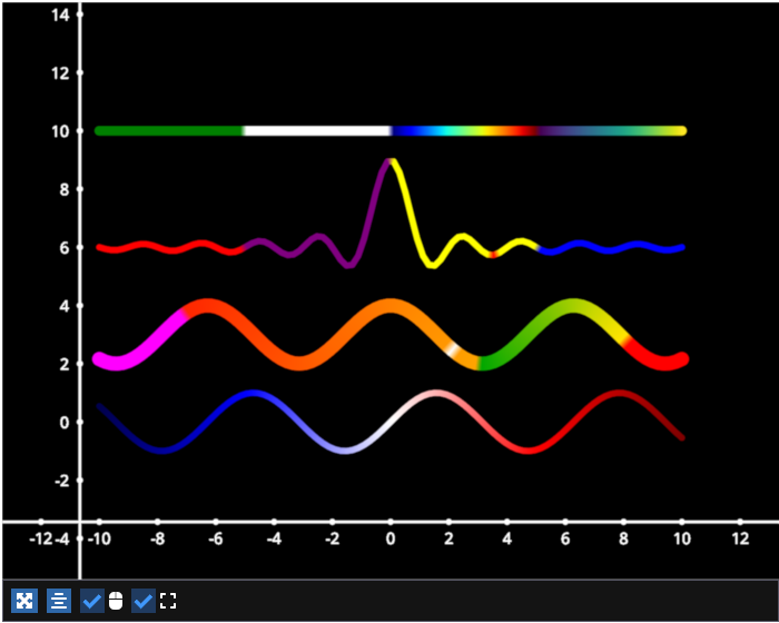
# test_example = true

import fastplotlib as fpl
import numpy as np

figure = fpl.Figure(size=(700, 560))

xs = np.linspace(-10, 10, 100)
# sine wave
ys = np.sin(xs)
sine_data = np.column_stack([xs, ys])

# cosine wave
ys = np.cos(xs)
cosine_data = np.column_stack([xs, ys])

# sinc function
a = 0.5
ys = np.sinc(xs) * 3
sinc_data = np.column_stack([xs, ys])

sine = figure[0, 0].add_line(
    data=sine_data,
    thickness=5,
    colors="magenta",
)

# per-vertex colors (same color initially) so we can slice into them below
cosine = figure[0, 0].add_line(
    data=cosine_data,
    thickness=12,
    colors=["orange"] * cosine_data.shape[0],
    offset=(0, 3, 0)  # places the graphic at a y-axis offset of 3, offsets don't affect data
)

# or a list of colors for each datapoint
colors = ["r"] * 25 + ["purple"] * 25 + ["y"] * 25 + ["b"] * 25
sinc = figure[0, 0].add_line(
    data=sinc_data,
    thickness=5,
    colors=colors,
    offset=(0, 6, 0)
)

zeros = np.zeros(xs.size)
zeros_data = np.column_stack([xs, zeros])
zeros = figure[0, 0].add_line(
    data=zeros_data,
    thickness=8,
    # per-vertex colors (same color initially) so we can change them individually later
    colors=["w"] * xs.size,
    offset=(0, 10, 0)
)

figure.show()

# indexing of colors
cosine.colors[:15] = "magenta"
cosine.colors[90:] = "red"
cosine.colors[60] = "w"

# more complex indexing, set the blue value directly from an array
cosine.colors[65:90, 0] = np.linspace(0, 1, 90 - 65)

# additional fancy indexing using numpy
key = np.array([0, 1, 2, 3, 4, 5, 6, 7, 8, 9, 10, 11, 12, 13, 14, 67, 19])
sinc.colors[key] = "Red"

# boolean fancy indexing
zeros.colors[xs < -5] = "green"

# assign a colormap to an entire line
sine.cmap = "seismic"


# NOTE: fpl.loop.run() should not be used for interactive sessions
# See the "JupyterLab and IPython" section in the user guide
if __name__ == "__main__":
    print(__doc__)
    fpl.loop.run()